From traces to experiments: A loop for improving AI agents

Let’s say your team shipped a support agent last quarter. The launch demo went well, stakeholders were pleased, and everyone moved on. A few months later, things start to look off. Summaries of long conversations are truncated, and monitors show latency spikes on tool calls to the billing API. Your team’s first instinct is to ship fixes such as tweaking prompts or upgrading the model. After the updates, performance seems to improve, but you still can’t tell why a change helped or whether it will hold as traffic changes.

The problem isn’t a lack of telemetry data. Teams that build and ship agentic systems usually capture more trace data than they can possibly review, but don’t have a repeatable way to identify where an agent is underperforming and measure whether a change improves the intended outcome.

In this post, we’ll cover how to read your agent traces as a roadmap for where to invest, why teams should run both evaluations and experiments, and how to bring them together into an optimization loop.

Use agent traces as a roadmap

Teams often look into traces when they need to debug bad interactions. Analyzing trace data in aggregate can reveal recurring patterns and show you where to invest next. When traces are connected to evaluation scores and outcomes, they can narrow vague concerns like “the agent could be better” into claims that are specific and testable, such as “our summarization prompt underperforms on threads over 15 messages, and those tickets reopen at twice the normal rate.”

A few types of signals are especially useful for getting to a hypothesis you can test:

• Latency patterns: When latency concentrates around one prompt or tool, it points to a potential bottleneck. If requests slow down whenever the billing tool fires, the model may be waiting on that tool call before it can respond.

• Cost anomalies: Expensive calls tend to cluster. Analyzing these groups can point you toward the cause. If the priciest traces correspond to long threads, the agent may be loading the full history into context on every turn. That pattern may point to unnecessary  context loading or a need to use a different model for those requests.

• Quality signals: These signals can reveal problems even when latency and cost look healthy. A response can have low latency and cost and still be wrong. Signals like eval scores, thumbs-down rates, escalation accuracy, and downstream reopens help you assess whether the agent is performing as intended. Tool-selection accuracy (did the agent pick the right tool for the task?) and tool-argument correctness (did the agent provide valid, complete arguments with the correct values for the task?) are especially important for agentic systems.

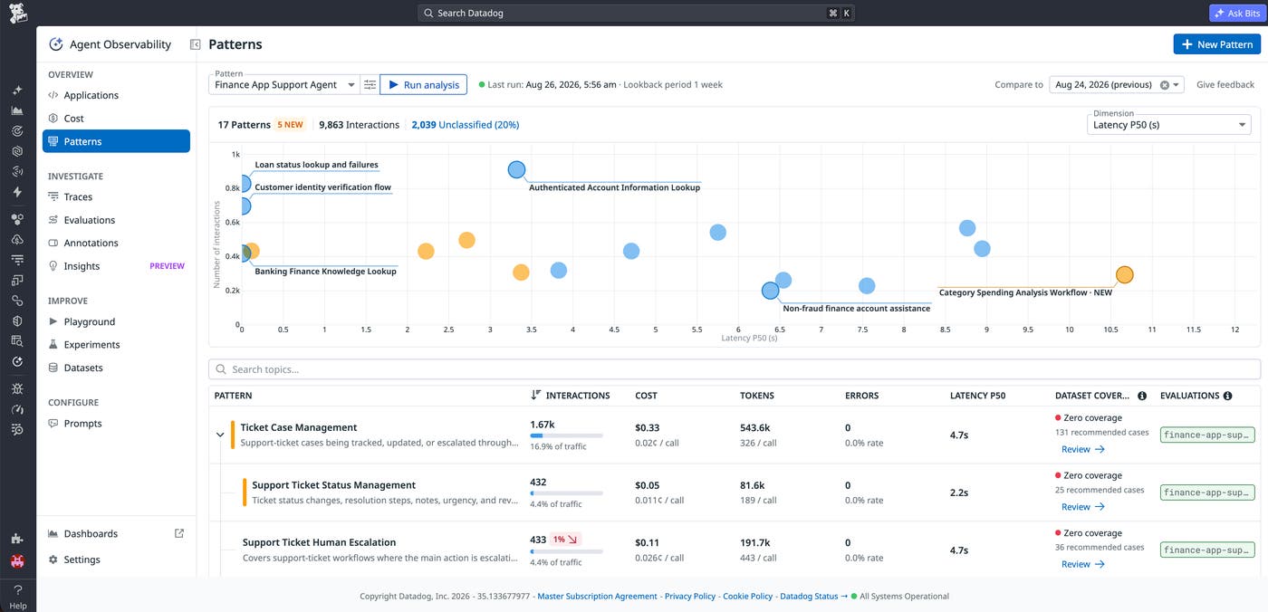
You can’t analyze and score interactions you never captured, so instrumentation must come first. Decide which quality dimensions you will prioritize, such as accuracy, policy adherence, and tone. Keep data granular enough to segment when diagnosing regressions, because a failure in one slice can disappear inside an average. Correlate traces with feedback and downstream outcomes, not just outputs. For a support agent, knowing that a ticket didn’t reopen tells you more than simply recording that the agent successfully replied.

Offline evaluation vs. online experimentation

Once the traces have pointed you toward a hypothesis, it’s time to test. Evaluation and experimentation answer different questions at different stages, and mature teams run both. Skip evaluation and you experiment on customers to learn what a dataset could have told you. Skip experimentation and you trust a test set that can break in production traffic. 

Evaluation runs a candidate change against a curated dataset of real scenarios, scored by evaluators, before any customer sees it. The goal is to find out whether the change clears your quality bar. No live traffic is required at this stage, but the same evaluators should run on a sample of production traffic after you ship to catch quality drift.

Experimentation tests whether a variant performs better than the baseline under the latency, cost, and traffic-distribution conditions that only production has. The goal here is to find out whether the change actually improves the outcome you care about for users or the business.

Evaluate first, then experiment. How much you should rely on each method depends on the scope of the change. For a small copy tweak on a prompt, evaluation with a light production check is usually enough. A model swap that touches every request deserves both a thorough offline benchmark and a staged rollout.

Building an optimization loop

Put those pieces together and you get a repeatable five-stage cycle: observe traces, form a hypothesis, evaluate offline, experiment in production, and keep monitoring after rollout. Each pass sharpens your datasets and evaluators, so the next one is faster and cheaper to run.

Observe

Start by picking one area of underperformance from the aggregate trace view. Analyze the data and focus on the segment with the worst outcomes, not the complaint you hear the most. For example: summary completeness averages 68% on threads over 15 messages, compared with 89% for shorter threads. Those tickets have a 12% reopen rate, compared with the overall baseline of 6%.

Hypothesize

The hypothesis that will drive the following steps must be specific enough to be wrong. “The summarizer seems bad on long tickets” is unhelpful because it doesn’t define what “better” looks like. A strong claim names four things: the proposed change, the segment, the primary metric, and the guardrails that must not regress.

For example: “For threads over 15 messages, switching to a map-reduce prompt will raise summary completeness from the 68% baseline to at least 83%. The variant must maintain a tone score of at least 90% and increase p95 latency by no more than 10%.” Change one variable at a time so you know what caused the result.

Evaluate offline

When running evaluations, use two separate datasets to answer different questions:

• A regression set, sampled to mirror production, that covers common scenarios and tells you whether overall performance moved.

• A coverage set that oversamples hard cases. This will tell you whether the edge cases you care about actually improved.

Score each set separately to keep the segmentation when it’s time to analyze the results. For tasks with a correct answer, give records ground truth. Use rubrics, outcome assertions, tool-call checks, human review or LLM-as-judge scoring for tasks that are subjective or have several valid outcomes.

Use the coverage set to ensure that important subgroups contain enough examples to assess independently, and report each subgroup’s results separately. Keep the regression set production-weighted so its aggregate score remains representative of normal traffic.

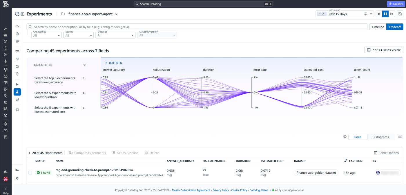
Reuse the same evaluators you’ll run in production, and calibrate any LLM-as-a-judge evaluator against human review before you rely on its scores. Run baseline versus variant on the identical dataset. For nondeterministic outputs, run each variant multiple times and compare the distribution of scores rather than relying on a single result from each version. Read deltas per evaluator and per segment to surface hidden regressions, such as a drop in the refund flow, before launch.

To keep LLM-as-a-judge costs manageable, score only a representative sample of records using the least expensive judge model that is reliable enough for the task. Plan this sampling strategy during the offline stage so the same evaluators remain affordable in production.

Experiment in production

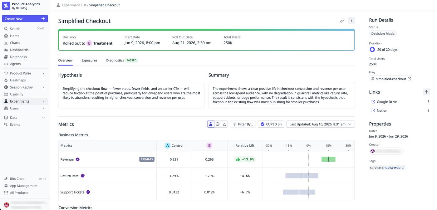
Promote only what cleared the offline bar. Before you start, define the success metric, guardrails, and decision rule. Split traffic with a feature flag, keep assignment sticky, and run until you hit your pre-committed stopping rule rather than stopping early because the primary metric looks good. Watch your guardrails (latency, cost, error rate, a secondary quality metric) so a win on the primary metric doesn’t hide regressions elsewhere.

Ship and keep watching

If the variant wins on the primary metric and stays within its guardrails, roll it out. Run the same evaluators on a sample of live traffic to confirm the win holds across the broader production distribution. When a new failure mode appears, add it to the dataset so the next evaluation cycle is stronger.

Over time, the loop produces better datasets and evaluators. After enough A/B tests, you can see which evaluators predicted the production outcome and which did not. Use that history to decide which ones to trust when choosing the next candidate to promote.

Close the AI experimentation loop in one place

When you use different tools for each stage of the AI experimentation loop, it’s harder to iterate smoothly. If traces live in one system, the offline evaluation bench in another, the A/B test behind a separate flag-and-analytics stack, and the dataset in an exported CSV, every iteration adds manual steps and opportunities for error. When observability and experimentation share a platform, signals flow directly into tests and the loop runs faster.

With Datadog, a trace that surfaces a problem in Agent Observability can become part of the dataset in Agent Observability Experiments for offline evaluation. After a candidate clears that stage, Feature Flags can serve the variants, while Experiments analyzes the online test against the selected outcome and guardrail metrics.

When you evaluate against real production data, it may contain customer personally identifiable information (PII) or other sensitive information. Scan and redact sensitive fields with Sensitive Data Scanner before you retain or reuse interactions for evaluation.

The loop closes when you test against production datasets before you ship, monitor quality drift in production, and feed those signals back into the next iteration.

Shipping verified improvements comes down to keeping traces, evaluations, and experiments connected as your agent scales. To learn more about running your own experiments with Datadog, check out our documentation. If you’re new to Datadog, get started with a 14-day free trial.