Homin Lee
It is essential to be able to spot unhealthy hosts anywhere in your infrastructure so that you can rapidly identify their causes and minimize service degradation and disruption. Discovering those misbehaving servers usually involves a careful study of how they perform normally and then setting threshold alerts on various metrics for each host.
As noted in the companion post announcing that outlier detection is now available within Datadog, threshold alerts can be difficult (or impossible) to define without setting off false alarms—particularly for metrics that are prone to spikes or whose baselines fluctuate. Instead, for these metrics, we should be taking advantage of a wealth of information available to us that we ignore when using simple threshold alerts: the metrics for all the healthy hosts.
Outlier detection works by comparing each host against the others in the group. Using our outlier detection algorithms, we can now alert when a host or group of hosts deviates from the pack, while avoiding alerts for expected, group-wide spikes:
We offer two different algorithms for this purpose: DBSCAN (density-based spatial clustering of applications with noise) and MAD (median absolute deviation). This post will discuss the technical details behind the two algorithms.
DBSCAN
A natural way to group together hosts that are behaving similarly is to use a clustering algorithm. We use DBSCAN, a popular density-based clustering algorithm, for this purpose. DBSCAN works by greedily agglomerating points that are close to each other. Clusters with few points in them are considered outliers.
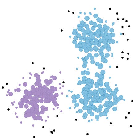
Traditionally, DBSCAN takes: 1) a parameter ε that specifies a distance threshold under which two points are considered to be close; and 2) the minimum number of points that have to be within a point’s ε-radius before that point can start agglomerating. The image below shows an example of DBSCAN in action on points in the plane. There are two clusters. The large points had enough close neighbors to agglomerate those points, while the small colored points did no agglomerating themselves but are within the ε-radius of a large point. The points in black are the outliers.
Parameters
We use a simplified form of DBSCAN to detect outliers on timeseries. We consider each host to be a point in d-dimensions, where d is the number of elements in the timeseries. Any point can agglomerate, and any point that is not in the largest cluster will be considered an outlier.
We set the initial distance threshold as follows. We create a new median timeseries by taking the median of the values from the existing timeseries at every time point across the selected time window. Then we calculate the (Euclidean) distance between each host and the median series. The threshold is the median of those distances, multiplied by a normalizing constant.
The only parameter we take is tolerance, the constant by which the initial threshold is multiplied to yield DBSCAN’s distance parameter ε. Here is DBSCAN with a tolerance of 3.0 in action on a pool of Cassandra workers:
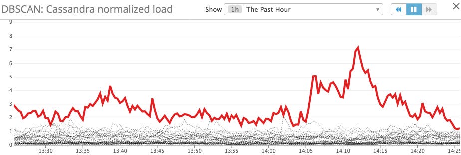
You should set the tolerance parameter depending on how similarly you expect your group of hosts to behave—larger values allow for more tolerance in how much a host can deviate from its peers.
MAD
The Median Absolute Deviation is a robust measure of variability, and can be viewed as the robust analogue for standard deviation. Robust statistics describe data in such a way that they are not unduly influenced by outliers.
For a given set of data D = {d<sub>1</sub>, ..., d<sub>n</sub>}, the deviations are the difference between each d<sub>i</sub> and median(D). The MAD is then the median of the absolute values of all the deviations. For example if D = {1, 2, 3, 4, 5, 6, 100}, then the median is 4, the deviations are {-3, -2, -1, 0, 1, 2, 96}, and the MAD is the median of {0, 1, 1, 2, 2, 3, 96}, which is 2. (Note that the standard deviation by contrast is 33.8.)
Parameters
In our case, the data set encompasses all points in every timeseries within the selected time window. We take the MAD of all the points, then multiply it by a normalizing constant and a tolerance parameter. The constant normalizes MAD so that it is comparable to the standard deviation of the normal distribution. The tolerance parameter then specifies how many “deviations” a point has to be away from the median for it to be considered an outlier.
Now, to mark a timeseries as an outlier, we use a second parameter, pct. If more than pct% of a particular series’ points are considered outliers, then the whole series is marked as an outlier. Here is MAD with a tolerance of 3 and pct of 20 in action when comparing the average system load by availability zone:

The tolerance parameter should be tuned depending on the expected variability of the data. For example, if the data is generally within a small range of values, then the tolerance should be small. On the other hand, if points can vary greatly, then you want a higher tolerance so that normal variabilities do not trigger a false positive.
DBSCAN vs. MAD
So which algorithm should you use? For most outliers, both algorithms will perform well at the default settings. However, there are subtle cases where one algorithm is more appropriate than the other.
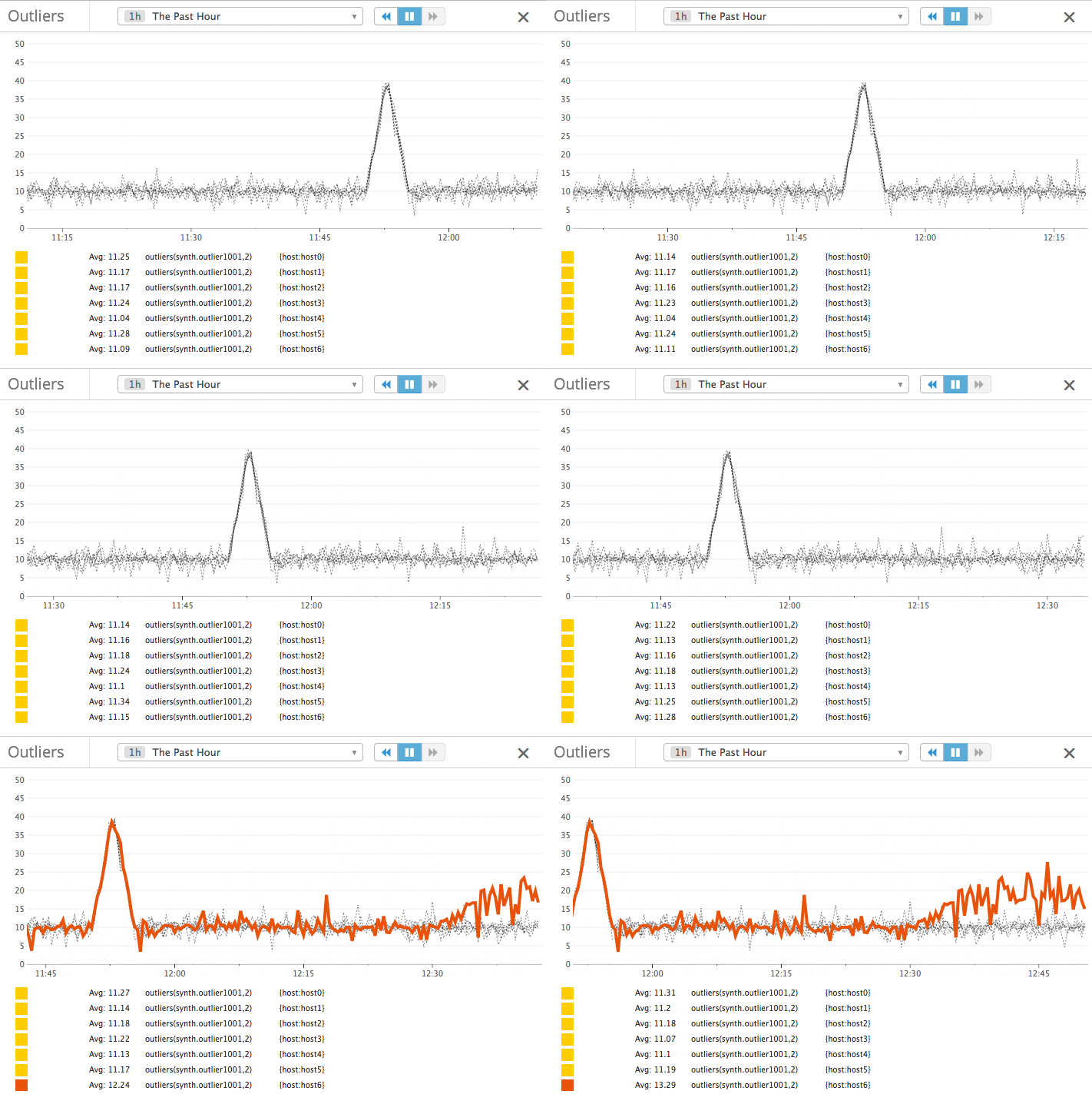
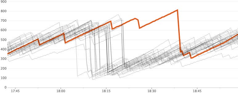
In the following image, we see a group of hosts flushing their buffers together while one host is flushing its buffer slightly later. DBSCAN picks this up as an outlier whereas MAD does not. This is a case where we would prefer to use MAD, as we don’t care about when the buffers get flushed. The synchronicity of the group is just an artifact of the hosts being restarted at the same time. On the other hand, if instead of flushed buffers, the metrics below represented a scheduled job that actually should be synchronized across hosts, then DBSCAN would be the right choice.
Setting up alerts
When setting up an outlier alert, an important parameter is the size of the time window analyzed. If the window is too large, by the time an outlier is detected, the bad behavior might have been going on for longer than one would like. If the window is too small, the alerts will not be as resilient to unimportant, one-off spikes.
Both algorithms are set up to identify outliers that differ from a majority of metrics that are behaving similarly. If your hosts exhibit “banding” behavior as shown below (perhaps because each band represents a different shard), we recommend tagging each band with an identifier, and setting up outlier detection alerts on each band separately.

What’s next
Outlier detection is just the first of the many algorithmic monitoring features we have coming down the pipeline. Stay tuned for more details as we roll out new tools to make your monitoring as dynamic as your infrastructure.
