Charles Masson
Designing powerful outlier and anomaly detection algorithms requires using the right tools. Discover how robust statistical distances can help.
Statistical distances are distances between distributions or samples, which are used in a variety of machine learning applications, such as anomaly and outlier detection, ordinal regression, and in generative adversarial networks (GANs). This post explores how to compare distributions using both visual tools and robust statistical distances.
When comparing data sets, statistical tests can tell you whether or not two data samples are likely to be generated by the same process or if they are related in some way. However, there are cases where, rather than deciding whether to reject a statistical hypothesis, you want to measure how similar or far apart the data sets are without any assumptions. Statistical distances, as distances between samples, are an interesting answer to that problem.
In this post, we'll cover:
Visual Inspection
Given two different sets of data, a quick visual inspection is often sufficient to compare their minimum and maximum values, their average values, and their spread. These are all features of their empirical distributions.
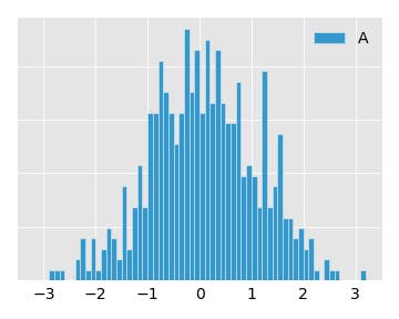
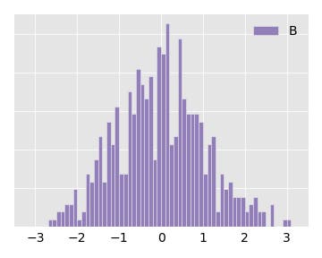
For example, these two data sets seem to have similar spread, and both are centered around 0. Looking at histograms of their values makes it seem like they're similarly distributed.
Q-Q plots are a handy tool for comparing distributions. Let's sort each data set by value, and then plot them against each other. The closer the values come to forming a straight line (the first bissector), the closer they are to coming from a similar distribution. The dots here indicate the 25th, 50th, and 75th percentiles.
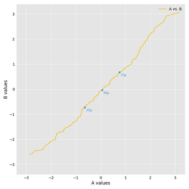
Given how their values lie close to a straight line, the Q-Q plot confirms what we've seen so far.
While visual inspection is a good heuristic to use, we often need a quantitative measure of the similarity between two distributions. I.e., we need to consider a distance between distributions.
Kolmogorov-Smirnov
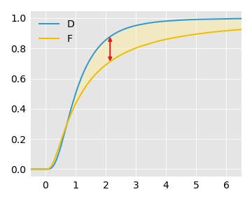
The first distance that we consider comes from the well-known Kolmogorov-Smirnov test (KS). To compare the two datasets, we construct their empirical cumulative distribution functions (CDF) by sorting each set and drawing a normalized step function that goes up at each data point. The KS distance is defined to be the largest absolute difference between the two empirical CDFs evaluated at any point.
In the case of
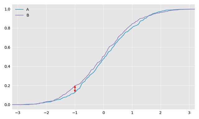
In fact, we can call it a distance, or metric>), because it satisfies four conditions that formalize the intuitive idea that we have of a distance:
its value is greater than or equal to zero,
it is equal to zero if and only if both distributions are identical,
it is symmetric: the distance from one distribution to another is equal to the distance from the latter to the former,
if
, and are distributions, then , or intuitively, with the definition of , it is shorter to go straight from to rather than going through , which is known as the triangle inequality.
Those properties make the KS distance powerful and convenient to use. Hence, given a third dataset
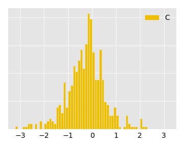
We have
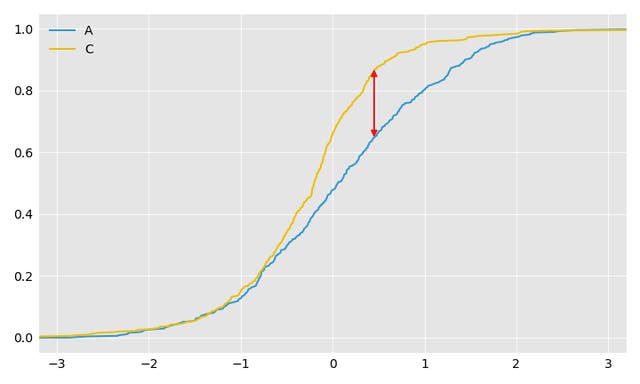
So we can immediately conclude that the KS distance between
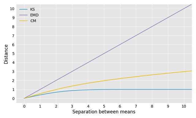
The KS distance is always between 0 and 1, so it is of limited use when comparing distributions that are far apart. For example, if you take two normal distributions with the same standard deviation but different means, the KS distance between them does not grow proportionally to the distance between their means:
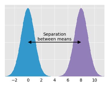
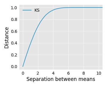
This feature of the KS distance can be useful if you are mostly interested in how similar your datasets are, and once it's clear that they're different you care less about exactly how different they are.
Earth Mover's Distance
Another interesting statistical distance is the Earth Mover's Distance (EMD), also known as the first Wasserstein distance. Its formal definition is a little technical, but its physical interpretation, which gives it its name, is easy to understand: imagine the two datasets to be piles of earth, and the goal is to move the first pile around to match the second. The Earth Mover's Distance is the minimum amount of work involved, where "amount of work" is the amount of earth you have to move multiplied by the distance you have to move it. The EMD can also be shown to be equal to the area between the two empirical CDFs.
The EMD is a good tool for distributions with long tails. Consider the following datasets
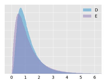
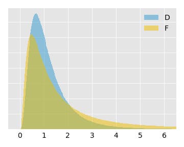
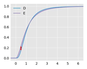
We calculate
Cramér-von Mises Distance
We can view the EMD as summing the absolute difference between the two empirical CDFs along the x-axis. The Cramér-von Mises (CM) distance is obtained by summing the squared difference between the two empirical CDFs along the x-axis (and then taking the square root of the sum to make it an actual distance). The relationship between the CM distance and the EMD is analogous to that of the L1 and L2 norms.
For the previous example
Let's consider again the example of two normal distributions with separated means. The EMD increases linearly as the means move farther away from each other, whereas the KS distance quickly levels off. The CM distance, on the other hand, grows like the square root function.
Illustrating the Properties of each Distance
Note that the KS distance is the maximum of the absolute difference between the CDFs whereas the EMD is the average absolute difference. This property makes KS much more sensitive to local deformations. This is also the reason why, when comparing a sample of data with a theoretical distribution, the KS test requires a large sample for accuracy.
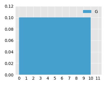
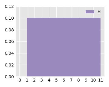
As an example, consider two uniform distributions
Here are their CDFs:
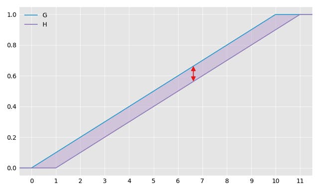
The distances between
, , .
Now, let's generate
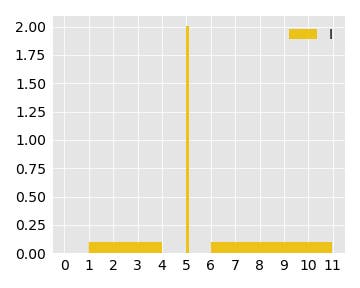
Here are the CDFs of
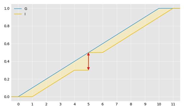
The distances between
, 100% higher than , , 0.2% higher, , 3.6% higher.
As we see, KS is highly affected by the deformation, whereas EMD is barely changed. CM seems to be a good tradeoff here, as it can still detect the deformation while not being excessively sensitive.
However, there are also deformations that do not affect KS but only EMD and CM. Consider the following distributions
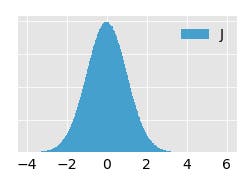
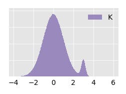
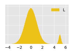
Visually, if you take
, .
Thus, the relative difference between the distances is only about 1% (71% for EMD, 39% for CM). We could slide the small bump farther to the right without affecting the KS distance at all. To understand how this can happen, let's consider the cumulative distribution functions of
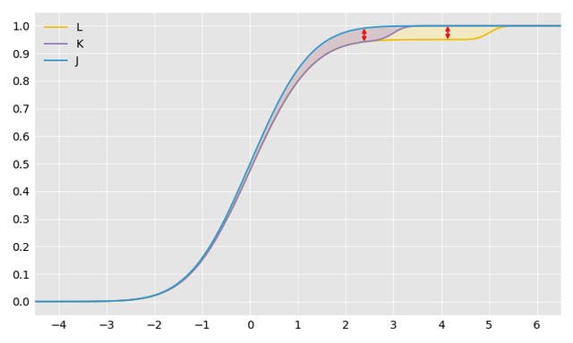
We see that by sliding the bump, we affect the CDF of
Try for Yourself!
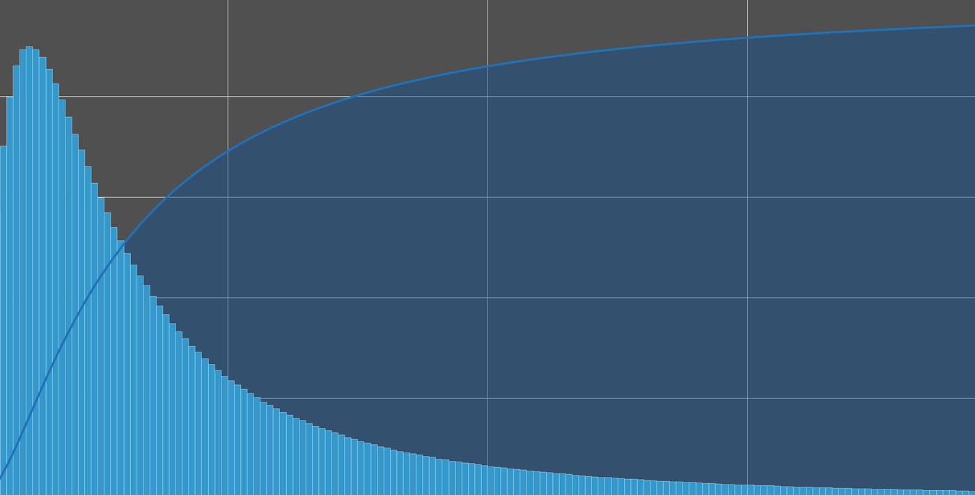
The interactive visualization at the top of the page lets you choose two distributions and generate two random samples of those distributions (of size 2000). You can then visualize their Q-Q plot and their CDFs, as well as the values of the Kolmogorov-Smirnov, the Earth Mover's and the Cramér-von Mises distances between both samples.
Code
All the methods discussed here have their place. There are plenty of plotting tools out there for conducting visual inspections, and the KS distance is widely implemented (for Python, Scipy has an implementation of KS). In July, we submitted an implementation of both the Earth Mover's Distance (also known as the first Wasserstein distance) and the energy distance (which is closely related to the Cramér-von Mises distance) as a Pull Request for inclusion in SciPy. The PR was recently merged and our implementations will be available in the next version of SciPy (namely version 1.0).
Notes
The Earth Mover's Distance generalizes nicely to multiple dimensions, but requires a primal-dual algorithm for computing the distance. The 2-dimensional case is often used in image processing.
There are actually two versions of the Cramér-von Mises distance:
the original non-distribution-free version, introduced by Cramér in 1928, which is the one that is considered here,
a distribution-free version, introduced by Smirnov in 1936, which is used for example in the Cramér-von Mises criterion.
The non-distribution-free version of the Cramér-von Mises distance is closely related to the energy distance, as its square equals
where , are independent random variables distributed according to one distribution and , are i.r.v. distributed according to the other. For those familiar with Fourier analysis, it should recall the Plancherel Theorem. However, calculating the distance from the CDF is much quicker. Cramér-von Mises has a weighted version called Anderson-Darling that's used as a test for determining if two distributions are the same or not. However, it is not a distance, and its value is highly sensitive to the sample size.
We only consider univariate distributions here, but if the dimension of your dataset is higher, and you only care to know if your two datasets are close or far apart, property testing becomes interesting. Clément Canonne wrote a nice technical survey (and an accompanying blogpost) on testing distributions.
