Stephen Kappel
Piecewise regression is a special type of linear regression that arises when a single line isn’t sufficient to model a data set. Piecewise regression breaks the domain into potentially many “segments” and fits a separate line through each one. For example, in the graphs below, a single line isn’t able to model the data as well as a piecewise regression with three lines:
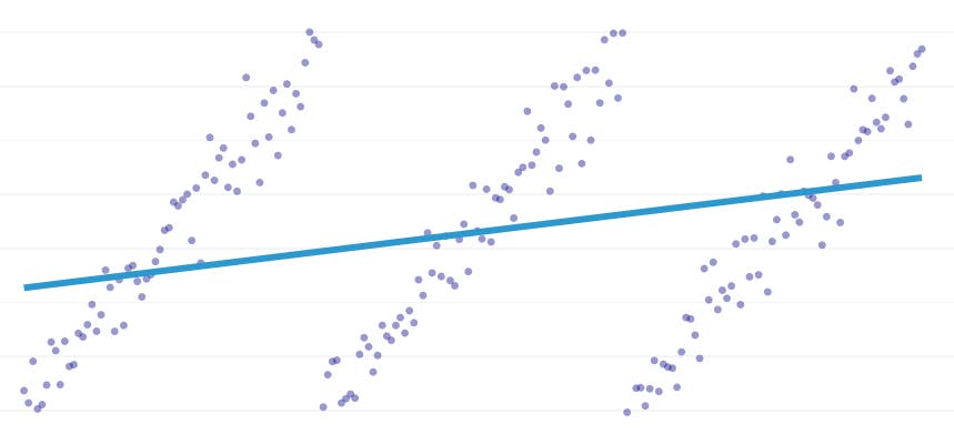
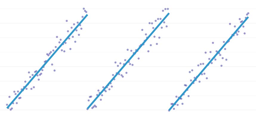
This post presents Datadog’s approach to automating piecewise regression on timeseries data.
Objectives
Piecewise regression can mean slightly different things in different contexts, so let’s take a minute to clarify what exactly we are trying to achieve with our piecewise regression algorithm.
Automated breakpoint detection. In classical statistics literature, piecewise regression is often suggested during manual regression analysis work, where it’s obvious to the naked eye where one linear trend gives way to another. In that case, a human can specify the breakpoint between piecewise segments, split the dataset, and perform a linear regression on each segment independently. In our use cases, we want to do hundreds of regressions per second, and it’s not feasible to have a human specify all breakpoints. Instead, we have the requirement that our piecewise regression algorithm identifies its own breakpoints.
Automated segment count detection. If we were to know that a data set has exactly two segments, we could easily look at each of the possible pairs of segments. However, in practice, when given an arbitrary timeseries, there’s no reason to believe that there must be more than one segment or less than 3 or 4 or 5. Our algorithm must choose an appropriate number of segments without it being user-specified.
No continuity requirement. Some methods for piecewise regressions generate connected segments, where each segment’s end point is the next segment’s start point. We impose no such requirement on our algorithm.
Challenges
The most obvious challenge to implementing a piecewise regression with automated breakpoint detection is the large size of the solution search space; a brute-force search of all the possible segments is prohibitively expensive. The number of ways a timeseries can be broken into segments is exponential in the length of the timeseries. While dynamic programming can be used to traverse this search space much more efficiently than a naive brute-force implementation, it’s still too slow in practice. A greedy heuristic will be needed to quickly discard large areas of the search space.
A more subtle challenge is that we need some way of comparing the quality of one solution to another. For our version of the problem, with unknown numbers and locations of segments, we need to compare potential solutions with different numbers of segments and different breakpoints. We find ourselves trying to balance two competing goals:
- Minimize the errors. That is, make each segment’s regression line close to the observed data points.
- Use the fewest number of segments that model the data well. We could always get zero error by creating a single segment for each point (or even one segment for every two points). Yet, that would defeat the whole point of doing a regression; we wouldn’t learn anything about the general relationship between a timestamp and its associated metric value, and we couldn’t easily use the result for interpolation or extrapolation.
Our solution
We use the following greedy algorithm for the piecewise regression problem:
- Do a piecewise regression with n/2 segments, where n is the number of observations in the timeseries. The regression line in each segment is fit using ordinary least squares (OLS) regression. This initial piecewise regression will have hardly any error, but it will severely overfit the data set.
- Iteratively, until there is only one segment:
- For all pairs of neighboring segments, evaluate the increase in total error that would result if the two segments were combined, their two regression lines being replaced by a single regression line.
- Merge together the pair of segments that would result in the smallest increase in error.
- If performing this merge meets our stopping criteria (defined below), then we might have gone too far, merging two segments that should remain separate. If this is the case, remember the state of the segments from before this iteration’s merge.
- If no merge resulted in remembering the state of segments in (2c) above, then the best solution is one large segment. Otherwise, the last segment state to be remembered in (2c) is the best solution.
Stopping Criteria
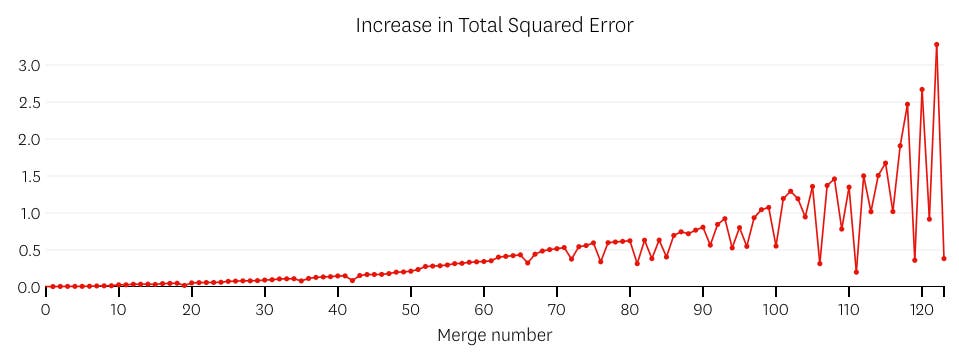
We consider a merge to be a potential stopping point if it increases the total sum of squared errors by more than any previous merge. To prevent stopping too soon in cases where there ought to be only one segment, we won’t consider a merge to be a potential stopping point unless it results in an increase in total error that’s less than 3% of the total error of a regression with one segment. (The 3% is an arbitrary threshold, but we have found it to work well in practice.) Below are a couple of examples to demonstrate why this stopping criteria works.
First, let’s look at a data set that was generated by adding normally-distributed noise to points along a single line. The algorithm correctly fits just a single segment through this data set.
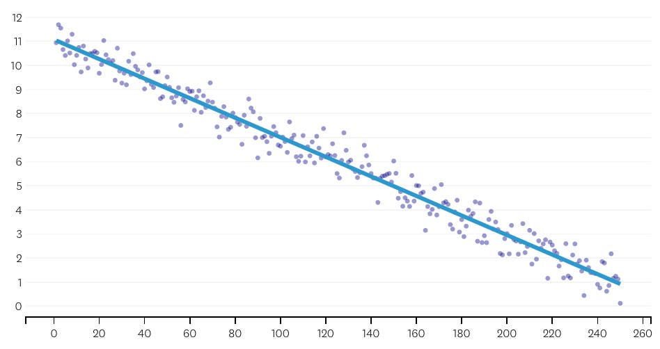
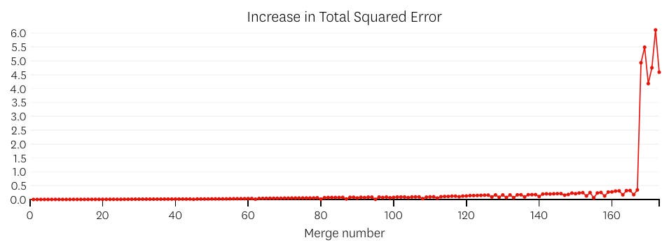
In this case, no merge ever increases the total sum of squared errors by more than 3%. Therefore, no merge is considered an adequate stopping point, and we use the final state after all merges have been executed. In the plot below, we see that later merges tend to introduce more error than earlier ones (which makes sense because they each impact more points), but the increase in error only gradually increases as more segments are merged.
Second, let’s look an example where there are seven distinct segment in the data set.
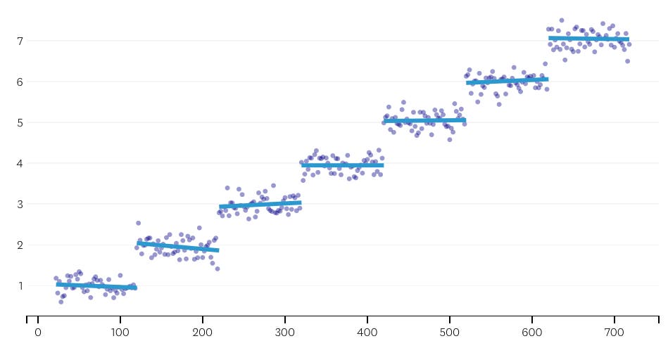
In this case, when we look at the plot of errors introduced by each merge, we see that the last six merges introduced much more error than any of the previous merges. Therefore, our algorithm remembered the state of the segments from before the 6th-to-last merge and used that as the final solution.
The code
In the Datadog/piecewise Github repo, you’ll find our Python implementation of the algorithm. The piecewise() function is where the heavy lifting happens; given a set of data, it will return the location and regression coefficients for each of the fitted segments.
Also included in the gist is plot_data_with_regression() — a wrapper function for quick and easy plotting. A quick example of how this might be used:
# Generate a short timeseries.t = np.arange(25)v = np.abs(t-7) + np.random.normal(0, 2, len(t))
# Fit a piecewise regression, and plot the result.plot_data_with_regression(t, v)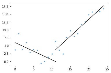
While this implementation uses OLS linear regression, the same framework can be adapted to solve related problems. By replacing squared error with absolute error or Huber loss, the regression can be made robust. Or, a step function can be fit by assigning each segment a constant value equal to the average of the observations in its domain.
